10 — Building an architecture you can read

Generated from a notebook

This page is notebooks/10_building_an_architecture.ipynb, executed, with its outputs. Run it yourself with jupyter lab notebooks/ after pip install 'somatize[viz]'. Interactive Plotly figures show here as the PNG the notebook also stores.

The three notebooks that follow are one story about one model.

10 (here)	Build the pipeline as a graph, and let the compiler tell you where the trainable region begins
11	Ask the model what is wrong with it before spending a sweep on it
12	Use what every run recorded to decide what to try next

The setting: a 1-D sensor stream with three regimes — a flat baseline, a slow drift, and a short burst. Two feature views, each deliberately blind to one of the three, and a model that has to combine them.

Everything is synthetic and seeded, so you can run this offline and get the same numbers.

import warnings

import numpy as np
import plotly.graph_objects as go
import plotly.io as pio
from IPython.display import SVG

import soma
from soma import Filter, Graph

pio.renderers.default = "plotly_mimetype+png"   # interactive here, PNG on GitHub
pio.renderers["png"].scale = 2
pio.renderers["png"].width = 950
warnings.filterwarnings("ignore", message="Full backward hook is firing")

import campaign   # the shared generator + filters, next to this notebook

10.1 — The stream

Three regimes over a 128-sample window. drift adds a slow rising ramp; burst adds a short high-frequency packet somewhere in the middle.

X, y = campaign.make_windows(512, seed=0)
Xtr, ytr, Xva, yva = campaign.split(X, y)

fig = go.Figure()
for cls, name in enumerate(campaign.CLASSES):
    fig.add_scatter(y=X[np.argmax(y == cls)], name=name, mode="lines")
fig.update_layout(
    title="One window per regime", height=320,
    xaxis_title="sample", yaxis_title="amplitude",
    margin=dict(t=48, b=40, l=48, r=16),
)
fig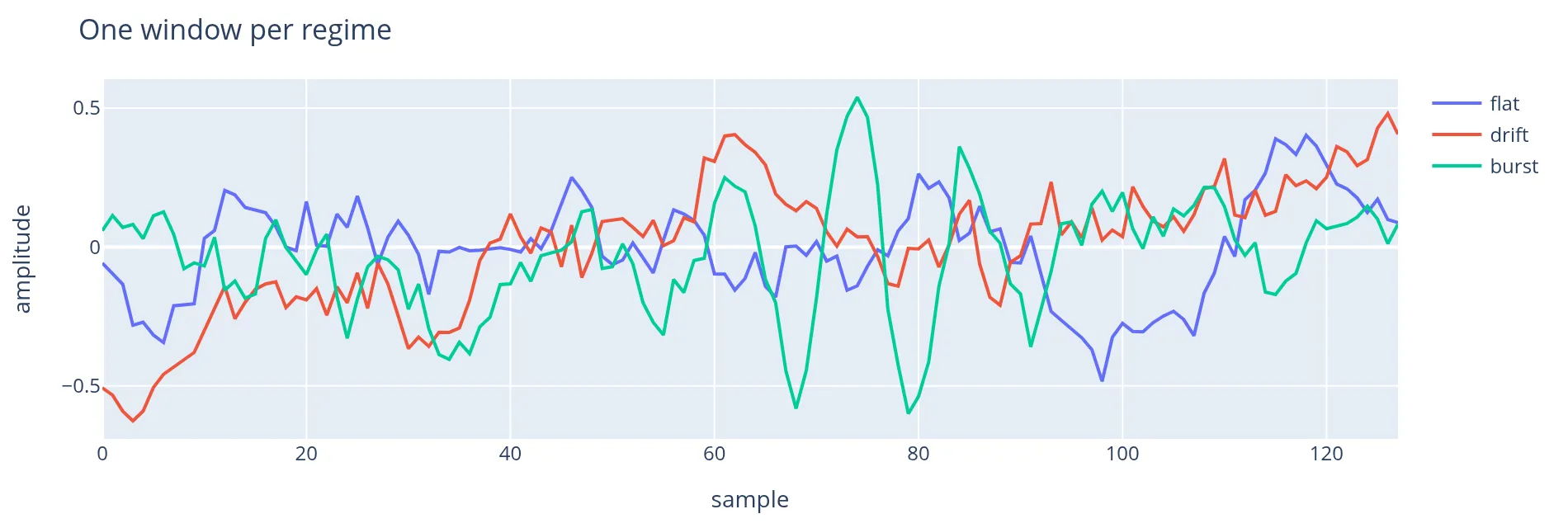

10.2 — Two views, each blind to one regime

The spectral view drops the lowest FFT bins — which is exactly where a linear drift puts its energy. The shape view mean-pools into 16 bins, which averages a fast oscillation away.

So neither view can classify all three regimes on its own. That is not a contrivance for the tutorial; it is the ordinary situation that makes a multi-branch model worth building, and in notebook 11 it is what makes a wiring bug between the branches cost something.

spec, shape = campaign.spectral_view(X), campaign.shape_view(X)

fig = go.Figure()
for cls, name in enumerate(campaign.CLASSES):
    fig.add_scatter(y=spec[y == cls].mean(0), name=f"{name} · spectral",
                    mode="lines", legendgroup="s")
    fig.add_scatter(y=shape[y == cls].mean(0), name=f"{name} · shape",
                    mode="lines", legendgroup="h", line=dict(dash="dot"), yaxis="y2")
fig.update_layout(
    title="Class means: the burst separates in the spectral view, the drift in the shape view",
    height=340, xaxis_title="feature index",
    yaxis=dict(title="log|rFFT|"), yaxis2=dict(title="pooled level", overlaying="y", side="right"),
    margin=dict(t=48, b=40, l=48, r=48),
)
fig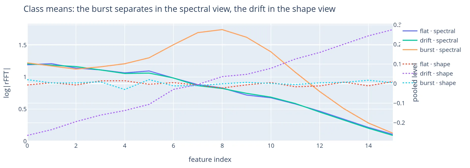

# A nearest-centroid probe: how much does each view carry alone?
def centroid_accuracy(F):
    tr, va = F[:384], F[384:]
    mu = np.stack([tr[ytr == k].mean(0) for k in range(3)])
    pred = np.argmin(((va[:, None, :] - mu[None]) ** 2).sum(-1), axis=1)
    return (pred == yva).mean()

for name, F in [("spectral only", spec), ("shape only", shape),
                ("both", campaign.features(X))]:
    print(f"{name:14s} {centroid_accuracy(F):.2f}")

spectral only  0.64
shape only     0.65
both           0.98

10.3 — Filters

A Filter is two methods. fit(x, y) learns state and returns it as a dict; forward(x, state) transforms. They are cached independently, so fit runs once per (configuration, data) and never again.

Filters defined in a notebook must declare _cache_version: a headless kernel has no source to hash, so without it soma falls back to cloudpickle and warns.

class Detrend(Filter):
    """Remove each window's linear trend — a stateless preprocessing step."""
    _cache_version = "nb10-detrend-v1"

    def fit(self, x, y=None):
        return {}

    def forward(self, x, state):
        a = np.asarray(x, dtype=float)
        t = np.linspace(-1, 1, a.shape[1])
        coef = (a * t).sum(1, keepdims=True) / (t * t).sum()
        return (a - coef * t).tolist()


class Spectral(Filter):
    _cache_version = "nb10-spectral-v1"

    def fit(self, x, y=None):
        return {}

    def forward(self, x, state):
        return campaign.spectral_view(np.asarray(x)).tolist()


class Shape(Filter):
    _cache_version = "nb10-shape-v1"

    def fit(self, x, y=None):
        return {}

    def forward(self, x, state):
        return campaign.shape_view(np.asarray(x)).tolist()


class Fuse(Filter):
    """Fan-in: `x` arrives as {node_id: branch_output}.

    Concatenated spectral-first, which fixes the channel layout that
    notebook 11's ChannelConfig.groups refers to by index.
    """
    _cache_version = "nb10-fuse-v1"

    def fit(self, x, y=None):
        return {}

    def forward(self, x, state):
        return np.concatenate([np.asarray(x["spectral"]),
                               np.asarray(x["shape"])], axis=1).tolist()


class Standardize(Filter):
    """The only fitted node: it learns the training mean and scale."""
    _cache_version = "nb10-standardize-v1"

    def fit(self, x, y=None):
        a = np.asarray(x, dtype=float)
        return {"mean": a.mean(0).tolist(), "std": (a.std(0) + 1e-9).tolist()}

    def forward(self, x, state):
        a = np.asarray(x, dtype=float)
        return ((a - np.asarray(state["mean"])) / np.asarray(state["std"])).tolist()

10.4 — The graph

>> chains, | forks, and a filter after a fork collects it.

The node ids come from the class names, lowercased — Spectral() becomes spectral. That is not cosmetic here: it is exactly the key Fuse reads out of its fan-in dict. Rename the class and you have renamed the key. (g.node("spectral", Spectral()) sets the id explicitly if you would rather not have that coupling; notebook 01 covers both forms.)

Evaluating the graph draws it.

g_prep = Graph.somatize(
    Detrend() >> (Spectral() | Shape()) >> Fuse() >> Standardize()
)
print(g_prep.filter_ids())
g_prep

['detrend', 'shape', 'spectral', 'fuse', 'standardize']

10.5 — Ask the compiler before you run

compile() reports what it can prove about the plan without executing it: how many nodes, how many are already cached, where the parallel branches are, and — in differentiable mode — every point where gradient flow is interrupted.

g_prep.compile(mode="differentiable")

nodes

5

cached

0

parallel branches

2

warning detrend

gradient flow interrupted at `detrend` (Trainable). Gradients from upstream will not reach downstream filters through this node.

info detrend

cache lookups are resolved at runtime per node (key = hash(config + state + input)); the compiled plan contains no Cached nodes

plan como texto

Sequence:
  Execute(detrend)
  Parallel:
    Execute(shape)
    Execute(spectral)
  Execute(fuse)
  Execute(standardize)

Every one of those diagnostics is correct: these are numpy filters, nothing here is differentiable, and a gradient could not cross any of them.

That is the argument for the split this notebook is building toward. Preprocessing is a fit-once, cache-forever stage; the trainable region starts after it. Keeping them in separate graphs means the sweep in notebook 11 and the four variants in notebook 12 all reuse one cached feature computation instead of recomputing it every time.

One more constraint worth knowing before notebook 11: the native training loop walks filters in topological order and threads one output into the next, so a differentiable graph has to be a chain. Branching still happens — inside a node, in its own nn.Module, which is exactly where DualViewEncoder puts it.

with g_prep.track_run("features", kind="fit", tags=["pulse-lab"]) as run:
    g_prep.fit(Xtr.tolist())
    Ftr = np.asarray(g_prep.forward(Xtr.tolist()))
    Fva = np.asarray(g_prep.forward(Xva.tolist()))

print("train features", Ftr.shape, " validation features", Fva.shape)
print("run:", run.id)

train features (384, 32)  validation features (128, 32)
run: run_20260804T003503_da2a

10.6 — The same graph, annotated with what happened

RunView reads the run directory. Nothing here re-runs anything — the diagram is the topology from graph.json with per-node timings, cache tiers and status folded in.

view = soma.RunView(run.dir)
SVG(view.to_svg())

view.plot_gantt()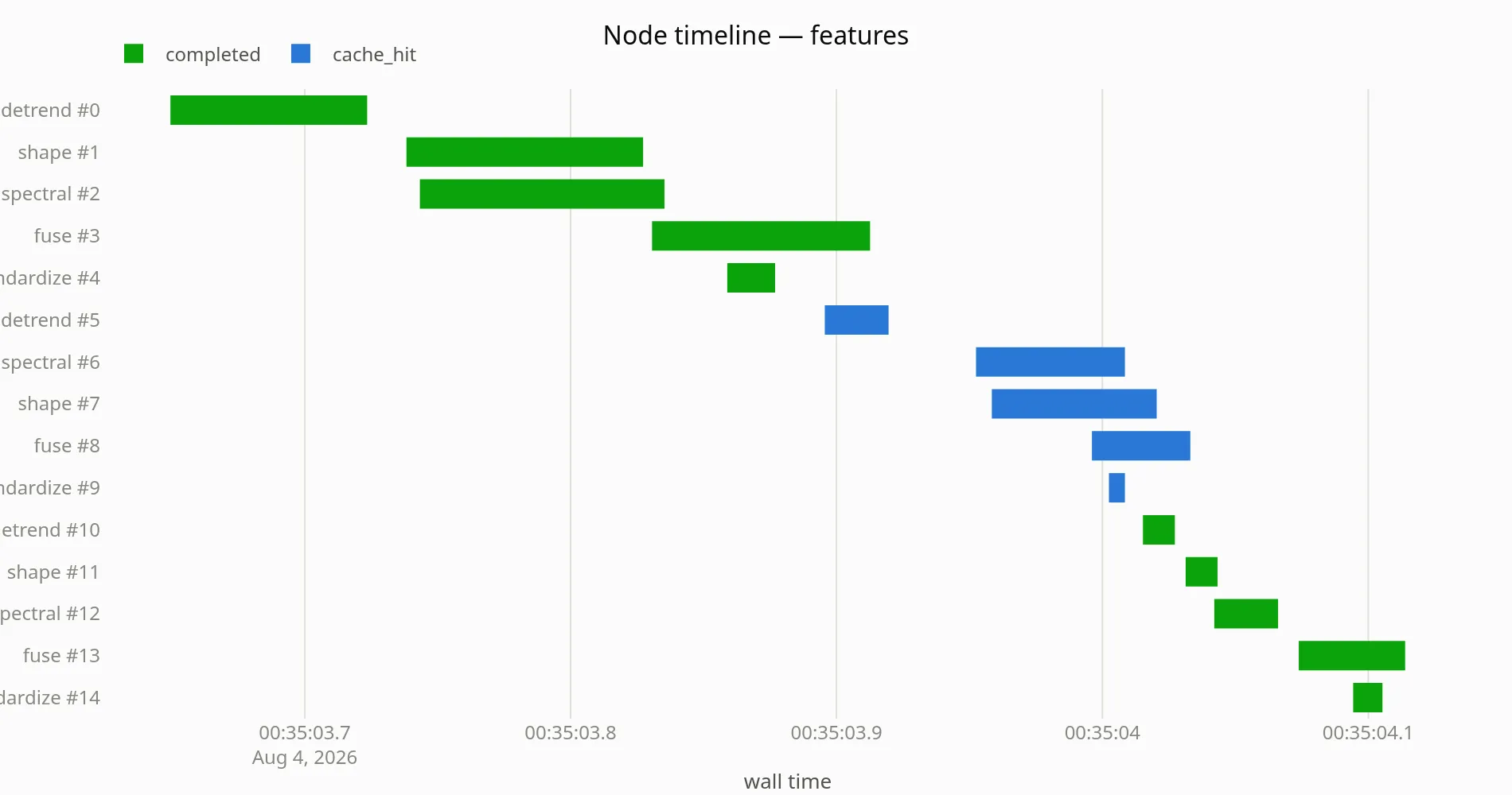

10.7 — The cache

Same configuration, same data, same result — and no recomputation. This is what pays for the sweep in notebook 11 and the variants in 12.

g2 = Graph.somatize(
    Detrend() >> (Spectral() | Shape()) >> Fuse() >> Standardize()
)

with g2.track_run("features-again", kind="fit", tags=["pulse-lab"]) as run2:
    g2.fit(Xtr.tolist())
    _ = g2.forward(Xtr.tolist())

activity = soma.RunView(run2.dir).cache_activity()
print(f"hits {activity['hits']}   misses {activity['misses']}")

hits 10   misses 0

soma.runs()

run id	kind	state	created	duration	name
run_20260804T003506_8975	fit	completed	2026-08-04 00:35:06	0.4s	features-again
run_20260804T003503_da2a	fit	completed	2026-08-04 00:35:03	0.6s	features

What’s next

Notebook 11 puts a model on top of these features — and finds four things wrong with it before tuning a single hyperparameter.